|
|
ContentsK-means
|
If your experience problems
with the applet start (it is possible because changes
starting with Java 7 Update 51),
you can download the applet here (kmeans.zip), save it on disk, unzip it
and start it by clicking on bat-file.
Please cite as: E.M. Mirkes, K-means and K-medoids applet. University of Leicester,
2011
Algorithms
K-means standard algorithm
The most common algorithm uses an iterative refinement technique. Due to its ubiquity it is often called the k-means algorithm; it is also referred to as Lloyd's algorithm, particularly in the computer science community.
Given an initial set of k means (centroids) m1(1),…,m k(1) (see below), the algorithm proceeds by alternating between two steps:
Assignment step : Assign each observation to the cluster with the closest mean (i.e. partition the observations according to the Voronoi diagram generated by the means).
![]()
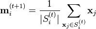
Update step : Calculate the new means to be the centroid of the observations in the cluster.
The algorithm is deemed to have converged when the assignments no longer change.
K-means is a classical partitioning technique of clustering that clusters the data set of n objects into k clusters with k known a priori. A useful tool for determining k is the silhouette.
K-medoids
The k-medoids algorithm is a clustering algorithm related to the k-means algorithm and the medoidshift algorithm. Both the k-means and k-medoids algorithms are partitional (breaking the dataset up into groups). K-means attempts to minimize the total squared error, while k-medoids minimizes the sum of dissimilarities between points labeled to be in a cluster and a point designated as the center of that cluster. In contrast to the k-means algorithm, k-medoids chooses datapoints as centers ( medoids or exemplars).
K-medoids is also a partitioning technique of clustering that clusters the data set of n objects into k clusters with k known a priori. A useful tool for determining k is the silhouette.
It could be more robust to noise and outliers as compared to k-means because it minimizes a sum of general pairwise dissimilarities instead of a sum of squared Euclidean distances. The possible choice of the dissimilarity function is very rich but in our applet we used the Euclidean distance.
A medoid of a finite dataset is a data point from this set, whose average dissimilarity to all the data points is minimal i.e. it is the most centrally located point in the set.
The most common realisation of k-medoid clustering is the Partitioning Around Medoids (PAM) algorithm and is as follows:
- Initialize: randomly select k of the n data points as the medoids
- Assignment step: Associate each data point to the closest medoid.
- Update step: For each medoid m and each data point o associated to m swap m and o and compute the total cost of the configuration (that is, the average dissimilarity of o to all the data points associated to m). Select the medoid o with the lowest cost of the configuration.
Repeat alternating steps 2 and 3 until there is no change in the assignments.
Brief guide for this applet
The applet contains three menu panels (top left), University of Leicester label (top right), work desk (center) and the label of the Attribution 3.0 Creative Commons publication license (bottom).
To wisit the web-site of the University of Leicester click on the University of Leicester logo.
To read the Creative Commons publication license click on the bottom license panel.
|
|
"Data set"
The first menu panel allows you to create and edit the data set. Every data point is displayed as a small circle on the work desk.
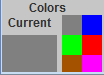
The first part of the Data set panel contains one big coloured rectangle and a palette built from six small differently coloured rectangles. To select one of the six colors click on a small rectangle. The big coloured rectangle displays the currently selected color.
The third part of the Data set panel contains six buttons. The first three buttons change the type of cursor brush.
The button "One point" switches the brush to add single points. Every mouse click on the work desk will add a point to the data set.
The button "Scatter" allows you to add several points by one mouse click. You can choose the number of added points in the "Number of points" spinner in the middle part of the menu panel. Points are scattered randomly in a circle whose radius is determined by the slider "Caliber" in the middle part of the menu panel.
The button "Erase" switches the mouse cursor in the eraser. When you click the eraser mouse cursor on the work desk, all points, whose centres are covered by the cursor, are removed from the work desk.
The button "Select" is not used
When you press the "Random" button several points are added on the work desk. The number of points is defined by the "Number of points" spinner. The locations of new points are generated randomly on whole work desk.
The button "Erase all" fully clears the work desk. It removes all kinds of object: data points, centroids, test results, maps and so on.
"Execution"
The second menu panel "Execution", is desined to initiate centroids and to learn models.
The leftmost part indicates the colour for for next added centroid. The user can not select centroid color.
The next part of the menu panel indicates the number of centroids, which can be added to the work desk.
|
|
There are two kinds of centroids: k-means centroids are four-ray stars and k-medoids centroids are nine-ray stars.
You can add centroids by the "Random centroid" button, or by clicking on a data point. Both centroids (k-means and k-medoids) are initialised simultaneously at the same data point.
The "Erase centroids" button allows you to remove ALL centroids.
Before you can see the results, you should press the "Learn" button.
After learning you can observe the results. If you want to edit centroids or the data set you should press the button "Unlearn".
"View learning history"
The third menu panel "View learning history" is needed to view the learning results. In the left top corner of the panel the number of steps is indicated that was needed to learn both models, and the number of the step showed in the work desk.
|
|
The leftmost button shows the first step. The second button moves to the previous step. The third button starts the slide show with one second delay between steps. It goes always from the first step to the last one. The fourth button moves to the next step. The rightmost button shows the last step.
The right part of menu panel are used to choose what is displayed on the work desk.
K-means only - the data set is coloured in accordance with k-means results. K-medoids centroids are not displayed.
K-means (show k-medoids centroids) - the data set is coloured in accordance with k-means results. Both groups of centroids are displayed.
K-medoids only - the data set is coloured in accordance with k-medoids results. K-means centroids are not displayed.
K-medoids (show k-means centroids) - the data set is coloured in accordance with k-medoids results. Both groups of centroids are displayed.