If your experience problems with the applet start (it is possible
because changes
starting with Java 7 Update 51),
you can download the applet here (PCASOM.zip), save it
on disk, unzip it and start it by clicking on bat-file.
Please cite as: E.M. Mirkes, Principal Component
Analysis and Self-Organizing Maps: applet. University of Leicester, 2011
First Play With PCA: go here to explore PCA with the applet
First Play With SOM and GSOM: go here to explore SOM and GSOM with the applet
Algorithms
Data points are xi (i=1,...,m). In the applet, they are situated on the 607×400 workdesk.
Principal component analysis
|
The first
principal component. |
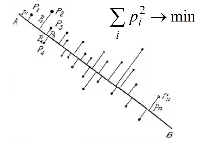
Principal component analysis (PCA) is the most popular method for data approximation by straight lines and planes, and for dimensionality reduction. PCA was invented by Karl Pearson. In 1901 he wrote: "In many physical, statistical, and biological investigations it is desirable to represent a system of points in plane, three, or higher dimensioned space by the "best-fitting" straight line or plane." The first principal component is the straight line that minimizes the sum of the squared distances from the data points. It is the least squares approximation of the data set by a line. The closest approximation is equivalent to the widest scattering of projections because of the Pythagorean theorem. Therefore, the first principal component maximizes the variance of projections of the data points on the straight line.To find the second principal component, it is sufficient to subtract from data vectors their projections on the first principal component and then find again the best straight line approximation, and so on. In this applet, we use the simple iterative splitting algorithm for calculation of the "best-fitting" straight line.
Two initial nodes, y1, y2, are defined by the user before learning. The data points xi (i=1,...,m) are given.
Algorithm
- Calculate the data mean X=(1/n)∑xi.
- Center data: xi←xi-X .
- Set k=0. Take initial approximation of the first principal component: v(0)=y2-y1.
- v(0)←v(0)/||v(0)|| - normalize v(0).
- Learning loop
- For each i from 1 to m calculate pi=(xi,v(k)) - calculate projection of the i-th point onto the current approximation of principal component.
- w=∑jxj pj - calculate direction of the next approximation. This w is proportional to the minimizer v in the problem ∑ j (xj - vpj)2→min
- v(k+1)←w/||w|| - normalize v(k+1).
- k←k+1 - next iteration.
- If (v(k-1),v(k))<0.99999 then go to step 5.1 (repeat the loop while the angle between two last approximations of the principal component is greater than 0.25°).
- v←v(k)
Further reading
- J. Shlens, A Tutorial on Principal Component Analysis: Derivation, Discussion and Singular Value Decomposition, 2003.
- A. N. Gorban, A. Y. Zinovyev, Principal Graphs and Manifolds, Chapter 2 in: Handbook of Research on Machine Learning Applications and Trends: Algorithms, Methods, and Techniques, Emilio Soria Olivas et al. (eds), IGI Global, Hershey, PA, USA, 2009, pp. 28-59.
- PCA for Pedestrian: Introductory Presentation
Self-organizing map
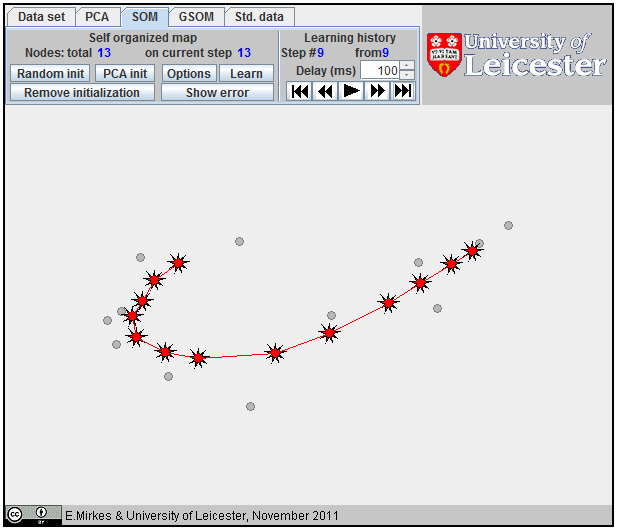
The Self-Organizing Map (SOM), also known as the Kohonen network, is a computational method for the visualization, low-dimensional approximation and analysis of high-dimensional data. It works with two spaces: a low-dimensional space with a regular grid of nodes and the higher-dimensional space of data. In our applet, the data space is two-dimensional (a plane) and the nodes form a one-dimensional array.
|
Radius 3 linear
B-spline |
Each node ni is mapped into the dataspace. Its image, yi is called the coding vector, the weight vector or the model vector. Rather often, the images of nodes in the data space are also called "nodes", with some abuse of language, and the same notation is often used for the nodes and the corresponding coding vectors. The exact sense is usually clear from the context.
The data point belongs to (or is associated with) the nearest coding vector. For each i we have to select data points owned by yi. Let the set of indices of these data points be Ci: Ci={l:||xl-yi||2≤||xl-yj||2 ∀i≠j} and |Ci| be the number of points in Ci.
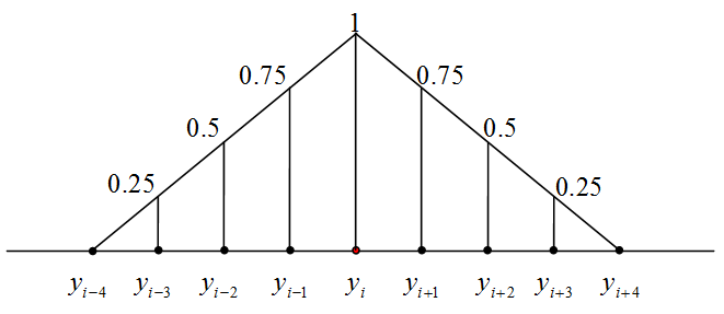
The learning of SOM is a special procedure that aims to improve the approximation of data by the coding vectors and, at the same time, approximately preserves the neighbourhood relations between nodes. If nodes are neighbours then the corresponding coding vectors should also be relatively close to each other. To improve the approximation of data, each coding vector yi moves during learning towards the mean point of the data points owned by yi. It involves in this movement the neighbours to preserve neighbourhood relations between nodes. This Batch SOM learning rule was proposed by Kohonen. The learning algorithm has one parameter, the "Neighbourhood radius" hmax. It is necessary to evaluate the neighbourhood function and this should be assigned before learning. For this applet, the neighbourhood function, hij, has the simple B-spline form: 1-hij=|i-j|/(hmax+1) if |i-j|=hmax and hij=0 if |i-j|>hmax (the example is given on the right).
|
1D SOM as a
broken line. |
The initial location of coding vectors should be assigned before the learning starts. There are three options for SOM initializations:
· The user can the select coding vectors randomly from datapoints;
· The coding vectors may be selected as a regular grid on the first principal component with the same variance;
· The coding vectors may be assigned manually, by mouse clicks.
All learning steps are saved into "Learning history". If learning restarts then the last record of Learning history is used instead of the user defined initial coding vectors.
Before learning, all Ci are set to the empty set (Ci=∅), and the steps counter is set to zero.
- Associate data points with nodes (form the list of indices Ci={l:||xl-yi||2≤ ||xl-yj||2 ∀i≠j}).
- If all sets Ci, evaluated at step 1 coincide with sets from the previous step of learning, then STOP.
- Add a new record to the learning history to place new coding vectors locations.
- For every node, calculate the sum of the associated data points: zi=∑j∈Cixj. If Ci=∅ then zi=0.
- Evaluate new locations of coding vectors.
- For each node, calculate the weight Wi=∑hij|Cj| (here, hij is the value of the neighbourhood function.)
- Calculate the sums Zi=∑hijzj.
- Calculate new positions of coding vectors: yiv←Zi/Wi if Wi≠0. If Wi=0 then yi does not change.
- Increment the step counter by 1.
- If the step counter is equal to 100, then STOP.
- Return to step 1.
If we connect the coding vectors for the nearest nodes by intervals then SOM is represented as a broken line in the data space. To evaluate the quality of approximation, we have to calculate the distance from the datapoints to the broken line and evaluate the Fraction of variance unexplained (FVU).
|
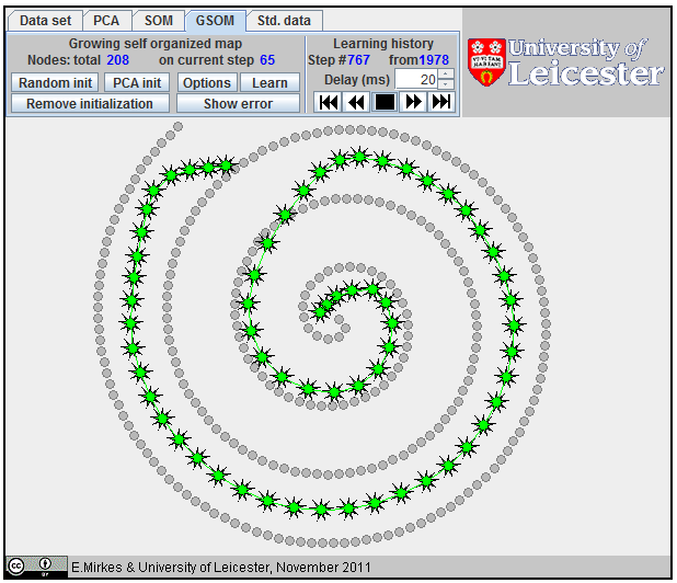
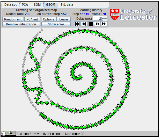
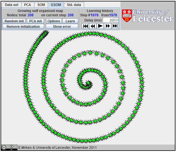
Approximation of a spiral by GSOM; 65 nodes,
Approximation of a spiral by GSOM; 152 nodes.
Approximation
of a spiral by GSOM.
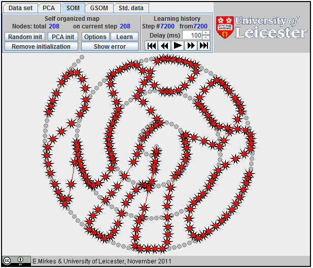
All attempts to
approximate a spiral by |
Further reading
- T. Kohonen and T. Honkela, Kohonen network (2007), Scholarpedia, 2(1):1568.
- H. Yin, Self-organising maps: Background, theories, extensions and applications, Computational Intelligence: A Compendium, Springer, 715-762, 2008.
- Self-organizing maps for WEKA: Implementation of Self-organizing maps in Java, for the WEKA Machine Learning Workbench.
- C. Ziesman, Self-Organizing Maps: Presentation for Beginners
Growing self-organizing map
The growing self-organizing map (GSOM) was developed to identify a suitable map size in the SOM. It starts with a minimal number of nodes and grows new nodes on the boundary based on a heuristic. At the same time, as a by-product, we can sometimes get better approximation properties (see an example on the right). There are many heuristics for GSOM growing. Our version is optimized for 1D GSOMs, the model of principal curves. GSOM method is specified by three parameters. Their values should be set before the learning starts:
· "Neighbourhood radius"
this parameter, hmax, is used to evaluate the neighbourhood function, hij (the same as for SOM).
· "Maximum number of nodes"
this parameter restricts the size of the map.
· "Stop when fraction of variance unexplained percent is less than..."
The threshold for FVU value.
The GSOM algorithm includes learning and growing phases. The learning phase is exactly the SOM leaning algorithm. The only difference is in the number of learning steps. For SOM we use 100 batch learning steps after each learning start or restart, whereas for GSOM we select 20 batch learning steps in a learning loop.
The initial location of coding vectors should be assigned before the learning starts. There are three options for GSOM initializations:
· The user can select coding vectors randomly from datapoints;
· The coding vectors may be selected as a regular grid on the first principal component with the same variance;
· The coding vectors may be assigned manually, by mouse clicks. We use n for the number of nodes in the map.
All learning steps (vectors yi) are saved into "Learning history". If learning restarts then yi from the last record of the Learning history are used instead of user defined initial coding vectors.
Beforethe start, set the step counter to zero and the sets of data points associated with nodes to the empty sets, Ci=∅.
- Calculate the variance of data (the base FVU)
- Learning loop.
- Associate data points with nodes (form the list of indices Ci={l:||xl-yi||2≤ ||xl-yj||2 ∀i≠j}).
- If all sets Ci, evaluated at step 2.1 coincide with the recorded sets from the previous learning iteration, then break the learning loop and go to step 3.
- Add new record to the learning history.
- For every node, calculate the sum of the associated data points: zi=∑j∈Cixj. If Ci=∅ then zi=0.
- Evaluate new locations of coding vectors.
- For each node, calculate the weight Wi=∑hij|Cj| (here, hij is the value of the neighbourhood function.)
- Calculate the sums Zi=∑hijzj.
- Calculate new positions of coding vectors: yiv←Zi/Wi if Wi≠0. If Wi=0 then yi does not change. Save in the learning history.
- Increment the step counter by 1.
- If the step counter is equal to 20, then break the learning loop and go to step 3.
- Return to step 2.1
- Check the termination criteria.
- If the number of nodes n is equal to the user defined maximum then STOP.
- Calculate FVU.
- If FVU is less than the user defined threshold then STOP.
- Map growing loop.
- If the map contains only one node then do:
- Add a new node and place a new coding vector at a randomly selected data point.
- Create a new learning history record. Save the old and new coding vectors into the record.
- If the map contains more than one node then do:
- Evaluate sets C1 and Cn associated with the first and the last node.
- If both sets, C1 and Cn, are empty then map growth is impossible and the growing loop is broken off; STOP.
- Evaluate the first node "quality" df=∑l∈C1||xl -y1||2.
- Evaluate the last node "quality" dl=∑l∈Cn||xl -yn||2.
- If df>dl then
- Create a new coding vector by attaching a copy of the first edge to the first coding vector y0=2y1 -y2.
- Evaluate FVUnew, that is FVU for the new set of coding vectors.
- If FVUnew < FVU then create a new learning history record, save the new set of coding vectors in the record, and continue learning from step 2. (Comment: The inequality FVUnew < FVU means here that at least for one data point the closest point on the new GSOM broken line is situated on the new semi-open segment [y0, y1).)
- Remove the new coding vector y0. Create a new coding vector, yn+1, by attaching a copy of the last edge to the last coding vector: yn+1=2yn -yn-1.
- Evaluate FVUnew, that is FVU for the new set of coding vectors.
- If FVUnew < FVU then create a new learning history record, save the new set of coding vectors in the record, and continue learning from step 2.
- Else STOP.
- If dl>df then
- Create a new coding vector by attaching a copy of the last edge to the last coding vector: yn+1=2yn -yn-1.
- Evaluate FVUnew, that is FVU for the new set of coding vectors.
- If FVUnew < FVU then create a new learning history record, save the new set of coding vectors in the record, and continue learning from step 2.
- Remove the new coding vector yn+1. Create a new coding vector, y0, by attaching a copy of the first edge to the first coding vector: y0=2y1 -y2.
- Evaluate FVUnew, that is FVU for the new set of coding vectors.
- If FVUnew < FVU then create a new learning history record, save the new set of coding vectors in the record, and continue learning from step 2.
- Else STOP.
- Go to step 2.
Further reading
- I. Valova, D. Beaton and D. MacLean SOMs for machine learning In: Machine Learning, Ed. by Y. Zhang, InTech, 2010, ISBN 978-953-307-033-9, pp. 20-44.
- D. Alahakoon, S. K. Halgamuge, and B. Srinivasan Dynamic Self-Organizing Maps with Controlled Growth for Knowledge Discovery. IEEE Transactions on Neural Networks 11 (3), (2000) 601-614.
- B. Fritzke, Kohonen Feature Maps and Growing Cell Structures - a Performance Comparison, Advances in Neural Information Processing Systems 5, [NIPS Conference], Morgan Kaufmann Publishers Inc. San Francisco, CA, USA (1993), pp.123-130, ISBN 1-55860-274-7. A gz archive of PS file or a PDF file from citeseerx. Some other papers of B. Fritzke.
Brief guide for this applet
The applet contains several menu panels (top left), the University of Leicester label (top right), work desk (center) and the label of the Attribution 3.0 Creative Commons publication license (bottom).
To wisit the web-site of the University of Leicester click on the University of Leicester logo.
To read the Creative Commons publication license click on the bottom license panel.
Data set
|
|
The first menu panel allows you to create and edit the data set. Every data point is displayed as a small circle on the work desk.
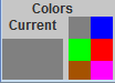
The first part of the Data set panel contains one big coloured rectangle and a palette built from six small differently coloured rectangles. To select one of the six colors click on a small rectangle. The big coloured rectangle displays the currently selected color. In this applet, this is just the colour of the cursor. The colours are used for data points in the applets K-means and K-medoids and KNN and Potential Energy to distinguish points from different classes and clusters.
The third part of the Data set panel contains six buttons. The first three buttons change the type of cursor brush.
· The button One point switches the brush to add single points. Every mouse click on the work desk will add a point to the data set.
· The button Scatter allows you to add several points by one mouse click. You can choose the number of added points in the Number of points spinner at the middle part of the menu panel. Points are scattered randomly in a circle which radius is determined by the slider Caliber in the middle part of menu panel.
· The button Erase switches the mouse cursor to the eraser. When you click the eraser mouse cursor on the work desk, all points, whose centres are covered by the cursor, are removed from the work desk.
· The button Select is not used in this applet.
· When you press the Random button several points are added on the work desk. The number of points is defined by the Number of points spinner. The locations of new points are generated randomly on whole work desk.
· The button Clear all completely clears the work desk. It removes all kinds of object: data points, centroids, test results, maps and so on.
Common parts of the menu panel for all methods
The All methods menu panel containes two parts.
|
|
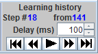
The right part, Learning history, contains five buttons, one field for data input and two information fields.
· The leftmost button shows the first step. The second button moves to the previous step.
· The third button starts the slide show with delay between steps selected in editable field Delay (ms). It goes always from the first step to the last one.
· The fourth button moves to the next step. The rightmost button shows the last step. The information field Step # shows the number of the current step.
· The information field from indicates the total number of learning steps in the learning history.
The left part of all methods menu panels contains the name of the method, two fields to show the number of nodes, and six standard buttons.
|
|
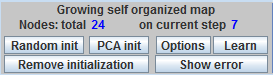
· The Random init button serves to add a coding vector at randomly selected data point to the current set of coding vectors.
· The PCA init button serves to add a new coding vector on the first principal conponent line. All coding vectors are distributed on the first principal component line equidistantly. The variance of this equidistribution on a segment is selected equal to the total variance of the data points.
· The Remove initialization button removes all nodes.
· The Options button opens options dialog for customizing method parameters. This dialog is specific for every method.
· The Learn button starts the learning process, specific for every method.
· The Show error/Hide error button shows/hides the tableau, which contains the names of the methods and the corresponding errors (Fraction of variance unexplained,). The tableau is located at the right bottom corner of the work desk.
PCA
Use the menu panel PCA to work with principal component analysis.
|
|
For PCA, all points and lines are in a blue color. The points for PCA have the form of four-ray stars (see left). To start PCA learning two points are needed. You can select initial points by mouse clicks at choosen locations, or by the button Random initialization. When you try add the third point, the first point is removed.
After learning is finished, use the Learning history buttons at the right part of menu panel to look at the learning history and results. You will see one four-ray star, the centroid of the data set, and one line, the current approximation of the first principal component.
SOM
Use the menu panel SOM to work with self organizing maps.
|
|
For SOM, all points and lines are in a red color. The points for SOM have the form of nine-ray stars (see left). To start SOM learning, the initial positions of all coding vectors are needed. To add a point to an initial approximation, click the mouse button at the choosen location, or use the button Random init or the button PCA init. When you add a new point, it is attached to the last added point.
After learning is finished, use the Learning history buttons at the right part of menu panel to look at the learning history and results.
GSOM
Use the menu panel GSOM to work with growing self organizing map.
|
|
For GSOM, all points and lines are in a green color. The points for GSOM have the form of nine-ray stars (see left). To start learning, GSOM is needed to initiate one point. To place initial point click the mouse button in the chosen location, or push the button Random init or the button PCA init. When you add a new point, the new point is joined with the last added point.
After learning is finished, use the Learning history buttons at the right part of menu panel to look at the learning history and results.
Std. data
The menu panel Std. data is needed to work with some standard data set.
|
|
· The first button Clear all comletely clears the work desk. It removes all kinds of objects: data points, coding vectors and so on.
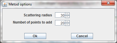
· The button Scatter serves to scatter existing data points. The scattering procedure adds a specified number of new data points in a specifyed circle around every data point, which exists. Options of scattering are defined in dialog (see left).
· The Number of points to add parameter defines the number of points to add to every data point.
· The Scattering radius parameter defines the radius of the circle around each data point where these new data points should be equidistributed.
· The last button Save data saves all data point locations to a text file named Data for mirkes.txt. In order to add this data set to the Std. data panel file with a short description you needed to send this file by e-mail to Evgeny Mirkes, emmirkes@gmail.com. Warning: To use the button Save data you should change settings of you browser security system, or start this applet off-line without brouser.
Any other button sends a stored ("standard") image to the work desk.
Fraction of variance unexplained
We approximate data by a straight line (PCA) or by a broken line (SOM and GSOM). The dimensionless least square evaluation of the error is the Fraction of variance unexplained (FVU). It is defined as the fraction:
[The sum of squared distances from data to the approximating line line/The sum of squared distances from data to the mean point].
The distance from a point to a straight line is the length of a perpendicular dropped from the point to the line. This definition allows us to evaluate FVU for PCA. For SOM and GSOM we need to solve the following problem. For the given array of coding vectors {yi} (i=1,2, ... m) we have to calculate the distance from each data point x to the broken line specified by a sequence of points {y1, y2, ... ym}. For the data point x, its projection onto the broken line is defined, that is, the closest point. The square of distance between the coding vector yi and the point x is di(x)=||x-yi||2 (i=1,2, ... m).
|
Projection of a data point onto a segment |
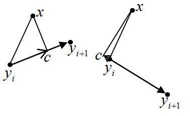
Let us calculate the squared distance from the data point x to the segment [yi, yi+1] (i=1,2, ... m-1). For each i, we calculate li(x)=(x-yi , yi+1-yi ) /||yi+1-yi||2 (see left).
If 0<li(x)<1 then the point, nearest to >x on the segment [yi, yi+1], is the internal point of the segment. Otherwise, this nearest point is one of the segment's ends.
Let 0<li(x)<1 and >c be a projection of x onto segment [yi, yi+1]. Then ||c - yi||2=(li(x)||yi-yi+1||)2 and, due to Pythagorean theorem, the squared distance from x to the segment [yi, yi+1] is ri(x)=||x-yi||2-(li(x) ||yi-yi+1||)2.
Let d(x)=min{di(x) | i=1,2, ... m} and r(x)=min{ri(x) | 0< li(x) <1, 0>< i< m }. Then the squared distance from x to the broken line specified by the sequence of points {y1, y2, ... ym} is D(x)=min{d(x), r(x)}.
For the given set of the data points xj and the given approximation by a broken line, the sum of the squared distances from the data points to the broken line is S=∑jD(xj), and the fraction of variance unexplained is S/V, where V=∑j(xj - X )2 and X is the empirical mean: X=(1/n)∑xi.